Reranking in RAG: Enhancing Accuracy with Cross-Encoders

Reranking has became a must-have in a Retrieval-Augmented Generation (RAG) stack. This powerful technique enables filtering results from a first retrieval step, greatly improving accuracy.

To understand reranking, we first need to take a look at encoders, and more precisely, bi-encoders and cross-encoders.

Encoder

Let’s first briefly explain what is an encoder. Since the introduction of the transformer architecture [Vaswani et al., 2017], a text encoder often refers to an encoder-only transformer such as BERT [Devlin et al., 2019]. It consists of a tokenizer, an embedding layer and then layers made of feed-forward networks and attention mechanisms. The attention mechanism attends both left and right context in all layers which enables to capture dependencies between tokens. This design allows the model to build rich contextualized representations of the input text, which is essential for many Natural Language Processing (NLP) tasks, including reranking.

Bi-Encoder

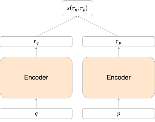
Bi-Encoder Architecture

The bi-encoder architecture consists of two separate encoders (in practice, it is often the same encoder used twice). These two encoders creates two compressed representations of the query and the passage: $r_q$ and $r_p$. To compute the relevance score between the query and the passage, a similarity function $s$ such as the dot product $s(r_q,r_p) = \langle r_q, r_p \rangle$ or the cosine similarity $s(r_q,r_p) = \frac{\langle r_q, r_p \rangle}{||r_q||.||r_p||}$ is applied.

Bi-Encoder Training

The training of a bi-encoder model aims to maximize the similarity between the query and the relevant passage while minimizing the similarity between the query and irrelevant passages. This is often achieved using a contrastive loss function, which encourages the model to push relevant pairs closer together in the embedding space and irrelevant pairs further apart.

In the case of one relevant passage and multiple irrelevant ones the contrastive loss $\mathcal{L}$ can be expressed as:

$$\mathcal{L}(q, p^+, (p_i^-)_i) = - \log \left( \frac{e^{\text{sim}(q, p^+)}}{e^{\text{sim}(q, p^+)} + \sum_{i=1}^n e^{\text{sim}(q, p_i^-)}} \right)$$

If there are multiple relevant passages and multiple irrelevant ones, it becomes:

$$\mathcal{L}(q, (p_j^+)_j, (p_i^-)_i) = - \log \left( \frac{\sum_{j=1}^m e^{\text{sim}(q, p_j^+)}}{\sum_{j=1}^m e^{\text{sim}(q, p_j^+)} + \sum_{i=1}^n e^{\text{sim}(q, p_i^-)}} \right)$$

where

• $q$ is the embedding of the query.
• $p^+$ is the embedding of the positive (relevant) passages.
• $(p_i^-)_i$ are the embeddings of the negative (irrelevant) passages.
• $(p_j^+)_j$ are the embeddings of the positive (relevant) passages, if there are multiple positive passages.
• $\text{sim}(q, p)$ is the similarity score between the query $q$ and passage embedding $p$ (typically a dot product or cosine similarity).
• $n$ is the number of negative samples.
• $m$ is the number of positive samples, if there are multiple positive samples.

Bi-Encoder Pros and Cons

One of the key advantages of bi-encoders is their efficiency. Since query and passage encodings can be precomputed independently, the retrieval phase requires only a simple similarity computation, which is almost instantaneous. This makes bi-encoders highly scalable, particularly suitable for large-scale retrieval tasks where millions of passages might need to be considered.

However, the downside is that the bi-encoder architecture may miss some fine-grained interactions between the query and passage because the representations are created independently. This limitation can lead to lower accuracy in cases where subtle semantic nuances matter.

Let’s see another encoder that is able to capture fine-grained interactions between the query and passage.

Cross-Encoder

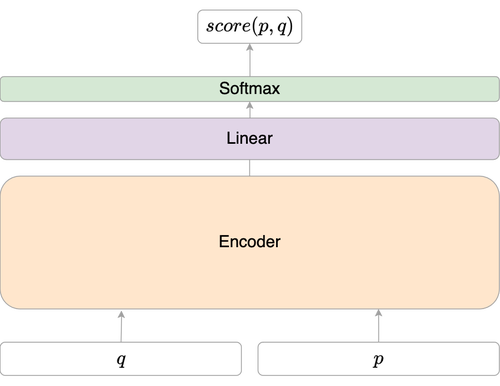
Cross-Encoder Architecture

In contrast to the bi-encoder, the cross-encoder architecture inputs both the query and passage together into a single BERT transformer. The attention mechanism is applied across the tokens of both sequences jointly, which allows the model to capture richer interactions between the query and passage. This architecture is known as an interaction model because it explicitly models the interaction between the two inputs at every layer of the transformer.

The fact that attention mechanism is able to attend both the query and the passage greatly improves accuracy.

Hence a cross-encoder is basically an encoder followed by a classifier. However we need to train it. Let’s see how.

Cross-Encoder Training

Cross-encoders are also trained to maximize and minimize the similarity between relevant and irrelevant query-passage pairs. To do so use use the Binary Cross-Entropy (BCE) loss which can be expressed as:

$$ \mathcal{L} = - \left( y \cdot \log(\hat{y}) + (1 - y) \cdot \log(1 - \hat{y}) \right) $$

where

• $y$ is the true label (1 for relevant, 0 for non-relevant).
• $\hat{y}$ is the predicted probability that the passage is relevant.

This loss function encourages the model to output higher probability for relevant query-passage pairs and lower probability for irrelevant pairs.

Cross-Encoder Pros and Cons

The cross-encoder’s ability to model the interactions between query and passage tokens allows for high accuracy, especially in tasks requiring nuanced understanding.

However, the need to recompute the encoding for each query-passage pair makes cross-encoders computationally intensive, particularly when working with large datasets. This limits their scalability compared to bi-encoders.

Indeed, if you have a query $q$ and some passages $P$.

• A bi-encoder would encode $q$ and compare it to the $|P|$ precomputed passages encodings. Hence, at inference, it requires 1 encoder forward pass.
• A cross-encoder would encode every pairs $(q,p), p \in P$. Hence, at inference, it requires $|P|$ cross-encoder forward passes.

Accuracy/scalability Trade-off

To achieve the best of both worlds, a common approach is to first perform a vector search using a bi-encoder, which quickly narrows down the candidate passages. The top candidates from this retrieval step are then reranked using a cross-encoder, providing a balance between efficiency and accuracy.

Even better, you can combine other retrieval techniques, such as BM25. This hybrid approach leverages the strengths of different models and avoids the need for a fusion formula like Reciprocal Rank Fusion (RRF), which blends scores from multiple retrieval models.

Conclusion

Reranking in a RAG stack effectively combines the scalability of bi-encoders with the accuracy of cross-encoders, offering a powerful tool for improving the relevance of retrieved information. As such, it plays a critical role in modern information retrieval and natural language processing systems.

References

• Passage Re-ranking with BERT
• Re2G: Retrieve, Rerank, Generate
• Reciprocal Rank Fusion outperforms Condorcet and individual Rank Learning Methods
• BERT: Pre-training of Deep Bidirectional Transformers for Language Understanding
• Attention Is All You Need

Further reading

• ColBERT: Efficient and Effective Passage Search via Contextualized Late Interaction over BERT
• What is ColBERT and Late Interaction and Why They Matter in Search?, Jina
• Late Chunking in Long-Context Embedding Models
• Hybrid Search Revamped